Temporal evolution of water quality at 1 m depth
[file = SondeHourly_270619-060720.csv , n = 12,366 observations].
The data presented are raw data, with an acquisition frequency of 30 min.
Table 1 - Data variability over the observation year (06/27/2019 to 06/07/2020). Variables: Temp = Temperature; Conductivity = Conductivity; ORP = Oxidation-reduction potential; DO = Dissolved Oxygen; Turbidity = Turbidity; RFU = Relative Fluorescence Unit; Chl-a = Chlorophyll-a, 1 RFU = 4 µg/L; BGA PC = Cyanobacterial Phycocyanin, 1 RFU = 1 µg/L; fDOM = Fluorescent Dissolved Organic Matter; Depth = Depth of water, 1 RFU = 1 µg/L; fDOM = Fluorescent Dissolved Organic Matter; Chl-a = Chlorophyll-a, 1 RFU = 4 µg/L. Depth = depth of the YSI EXO2 probe, Statistics: Mean = Mean; Max = Maximum; Min = Minimum; Median = Median; Stdev = Standard deviation; SE = Standard error (= Stdev/root(number of observations)). *PH sensor decalibrated during the first months. Replaced on 02/12/2019 as of which values are reliable. **Outlier ORP value. Reliable DO values as of October. ***Because the YSI EXO2 sonde remained more than 2 months on the bottom (~10 m), the average depth is 4.15 m, however its average is 0.97 m, or corresponds to the 1.0 m programmed.

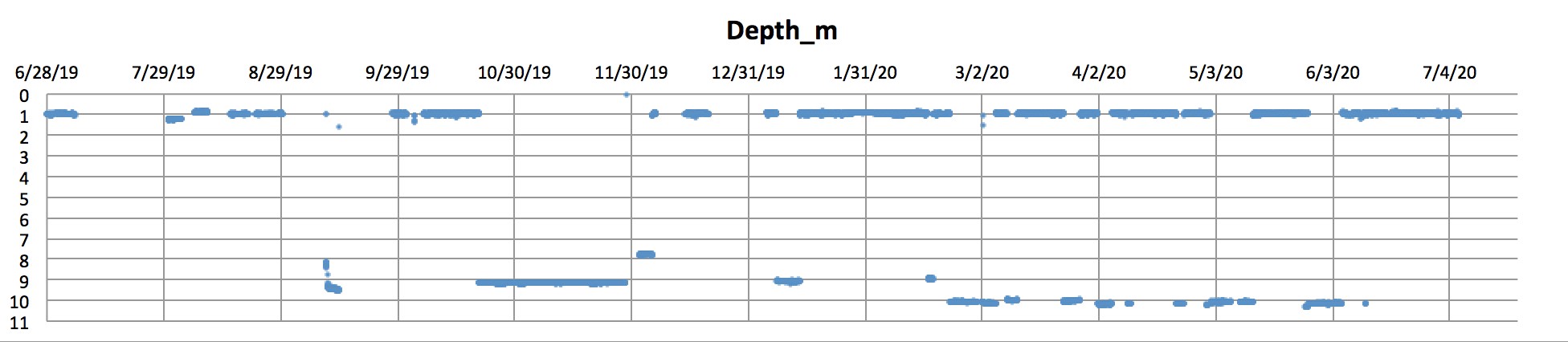
Figure 1 - Time evolution of the YSI EXO2 sonde immersion depth (programmed at 1 m depth to take measurements at every 30 min) during the monitoring period. On several occasions the sonde remained close to the bottom (retained by drifting fishing nets; or for unknown reasons; need to be attentive to send the sonde to the surface and program it to start the profiles again). Since June 2020, it did not happen anymore. Care must be taken to interpret the data.
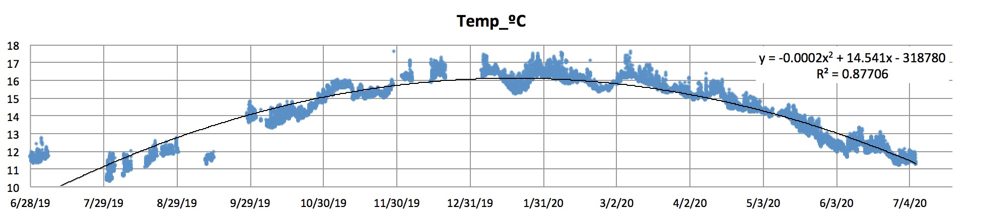
Figure 2 - Time evolution of the water temperature at 1 m depth (except for the periods during which the sonde was at the bottom; see previous figure). The temperature follows a perfectly parabolic curve , with a maximum of 17 ºC at the end of January, and a minimum of 11ºC in July. Note: dates follow the month/day/year format.

Figure 3 - Temporal evolution of conductivity (in µS/cm). On average it remains at 1,455 µS/cm, except between October and November when the YSI EXO2 sonde was trapped at the bottom, reaching 1,176-1,258 µS/cm (not visible on the graph). This may suggests the presence of fresher water at the bottom.
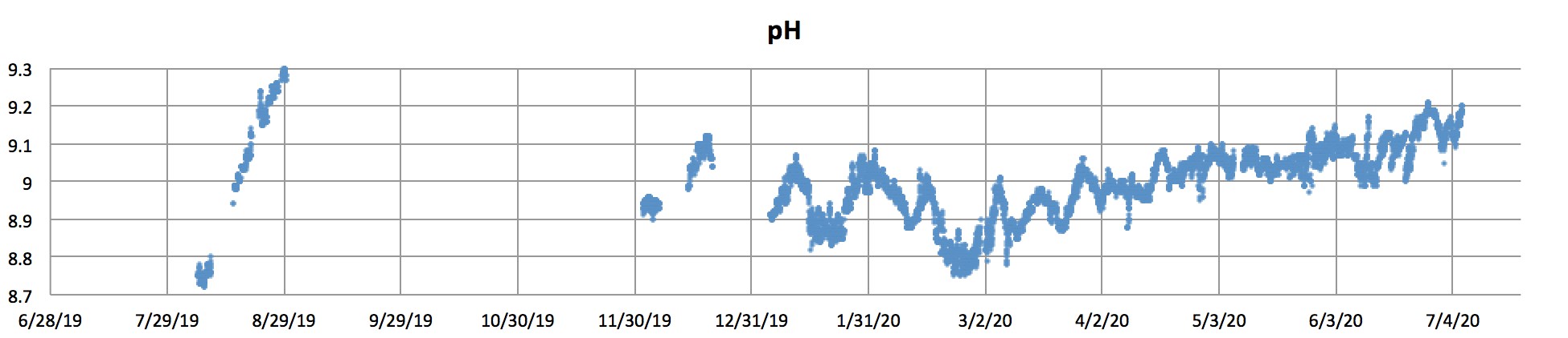
Figure 4 - Temporal evolution of pH. From June to November, we had a decalibrated sensor (its drift is observed) that was replaced by a new one on 0/12/2019, from when the measurements were reliable.The pH fluctuated between 8.75 and 9.21, with an average of 9.00.
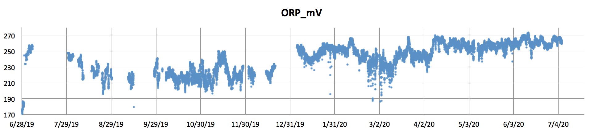
Figure 5 - Time evolution of the oxidation-reduction potential (ORP) in millivolts. The sensor was recalibrated in October. However, the data are reliable from December onwards when they fluctuate between 190 and 270 mV, being 241 mV on average.

Figure 6 - Temporal evolution of the dissolved oxygen saturation percentage. The sensor was recalibrated in October. From January, it fluctuated between 67 and 114%, with an average of 98%. This behavior represents a very good level of oxygenation, in equilibrium with the atmosphere. Cycles (oscillations) of 2-4 weeks are observed.
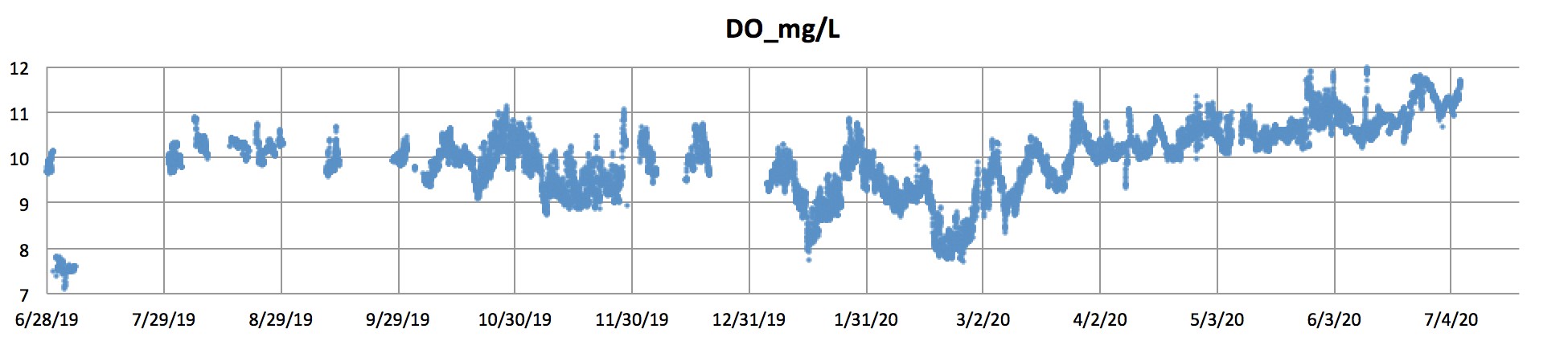
Figure 7 - Temporal evolution of dissolved oxygen concentration. For the same reason, the data are reliable from October onwards. From October to December it fluctuates between 8.5 and 11.0 mg/L. From January it fluctuates between 7.5 and 11.0 mg/L, with periods of 2-4 weeks. From March onwards, it gradually increases up to 12.0 mg/L in June. Corresponds to a good level of oxygenation, given the altitude of the lake.
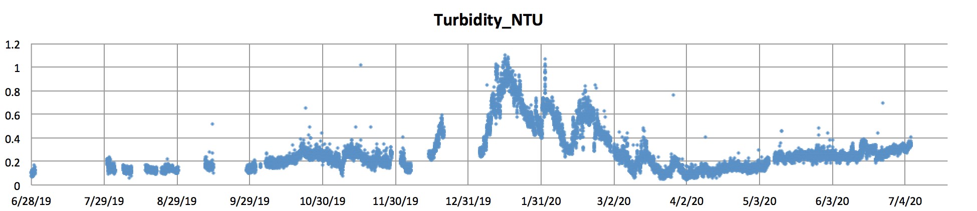
Figure 8 - Temporal evolution of turbidity. During the dry period (until November) it remains between 0.1-0.4 NTU. It increases in the rainy period (December-February). From January on, it reached 1.1 NTU, then gradually decreased with oscillations until reaching 0.1-0.2 NTU at the end of March. From June onwards, it increased slightly. The average is 0.28 NTU, with fluctuations between 0.08 and 4.02 NTU. So the water is very clear. It can be noted that the pattern of turbidity evolution follows the pattern of chlorophyll-a concentration (Fig. 9). In other words, turbidity results mainly from the phytoplankton biomass(not suspended mineral particles).
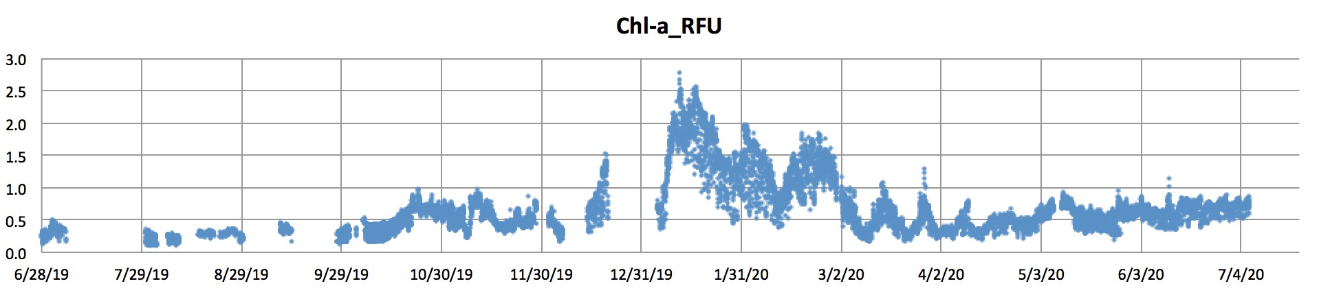
Figure 9 - Temporal evolution of total chlorophyll-a concentration (in RFU). In the dry period, it remains between 0.2-1.0 RFU (according to the calibration with the FluoroProbe bbe presented in Annex 5 of the 5th Quarterly Report, the NTU x 8.0 one has to multiply the NTU x 8 to convert to µg/L), i.e. equivalent to 1.6-8.0 µg/L (oligotrophic to mesotrophic). During the rainy period in January-February (due to nutrient inputs from river wastewater, in addition to atmospheric inputs from aerosols) it increases between 0.5-2.8 RFU, i.e. equivalent to 4.0-22.4 µg/L (predominantly mesotrophic-eutrophic). During the annual cycle, chlorophyll-a fluctuated between 0.10 and 2.78 NTU (i.e. 0.80 and 22.24 µg/L), with an average of 0.69 NTU (i.e. 5.52 µg/L). In comparison, during 1979-1980, for all of Minor Lake, chlorophyll-a concentrations did not exceed 0.5 µg/L during the dry period and 2.0 µg/L in the rainy period, with a maximum of 5.0 µg/L (Lazzaro, 1981).
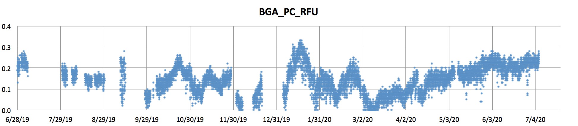
Figure 10 - Temporal evolution of the concentration of phycocyanin (photosynthetic pigment of cyanobacteria). During this period it remains below 0.35 RFU, with a maximum of 1.72 RFU. According to the calibration of the manufacturer YSI, 1 RFU = 1 µg/L phycocyanin. The average is 0.14 RFU (=0.14 µg/L) that is a very low concentration. The concentration was highest in January, and increased gradually from April onwards.
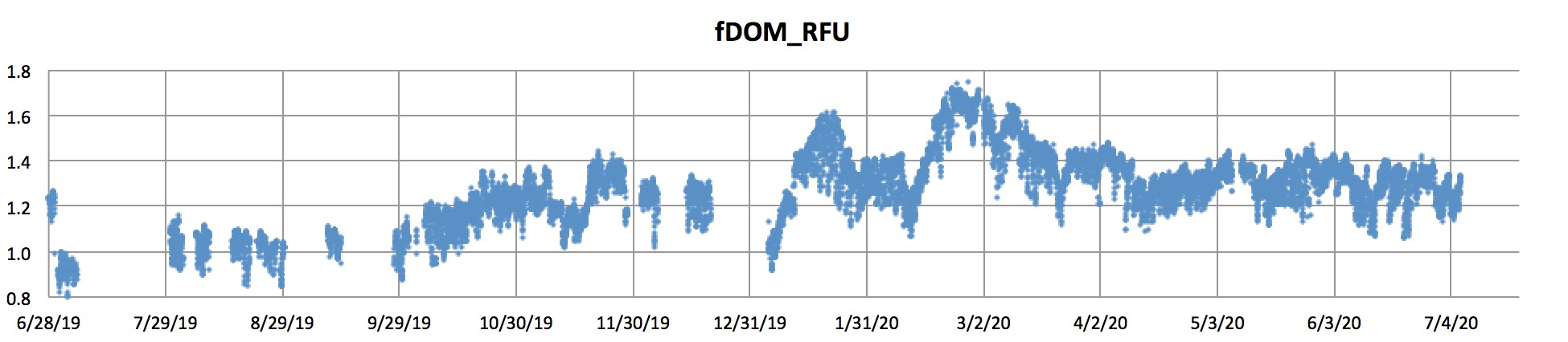
Figure 11 - Temporal evolution of the fluorescent dissolved organic matter (fDOM) concentration. During the dry period it varied between 0.8-1.4 RFU. Slight increase during the rainy period from January 2020 onwards, up to 1.8 RFU. This increase in January and February resulted from organic matter inputs from the rivers, particularly from the Katari basin, via the Cohana and Sehuenca rivers. Cohana and Sehuenca rivers joining in Cumana Lagoon, which flows into Cumana Bay. As of March, it stabilized around 1.3 RFU.
Temporal evolution of water quality along vertical profiles between 1 and 10 m depth every 2 hours
[file = PFL_Step_270619-060720.csv , n = 22,241 observations].
The time scale (horizontal axis) of the graphs is indicated with monthly divisions.
Table 2 - Variability of data over the observation year (06/27/2019 to 07/06/2020). For variable abbreviations and statistics see Table 1.
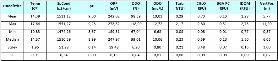

Figure 12 - Vertical profiles at every meter between 1 and 10 m depth performed every two hours (2:00, 4:00, 6:00, ..., 22:00, 24:00; i.e. 12 daily profiles). On several occasions the probe was trapped near or on the bottom dragged by drifting fishing nets, or for unknown reasons as the last time between 27/05 and 05/06/2020. As the missions were forbidden since March, the causes could not be determined.
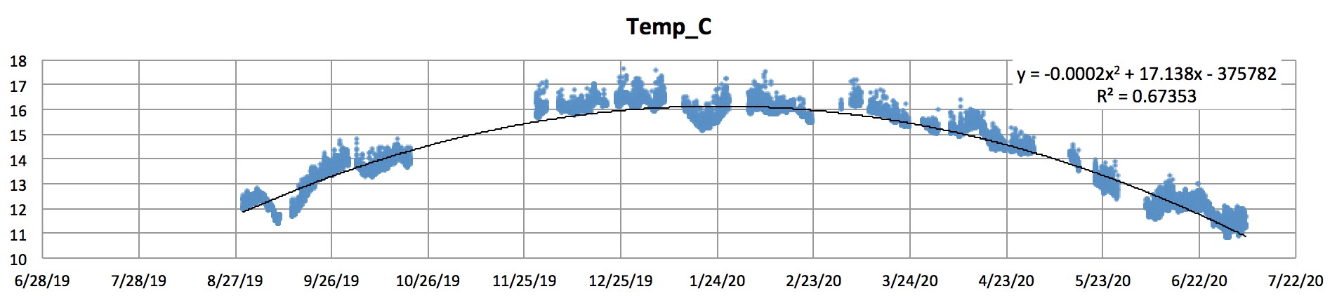
Figure 13 - Time evolution of vertical temperature profiles between 0 and 10 m depth. The data follow a parabola curve (in relation to the seasonal variation of the height of the sun on the horizon). From September 2019, the temperature increased from 11.0 ºC to a maximum of 17.5 ºC in January-February, then decreased to 11.0 ºC in June 2020. From December onwards, it remains between 15.0 and 17.0 between 15.0 and 17.5 ºC. The daily vertical variability is low at around 1.0-1.5 ºC.

Figure 14 - Evolution of conductivity, which varies slightly between a minimum of 1480 in February and a maximum of 1540 µS/cm on January 2, 2020. The conductivity drops towards ≤ 1500 µS/cm during the rainy season (January-February).
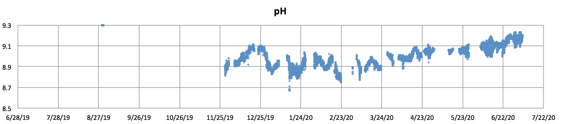
Figure 15 - pH evolution. We only installed a calibrated sensor on November 27th. So the data are only valid from December onwards. The average pH was 9.0 and varied very little between 8.7 and 9.2, with little variation, with very little vertical variability (≤ 0.1 pH unit).
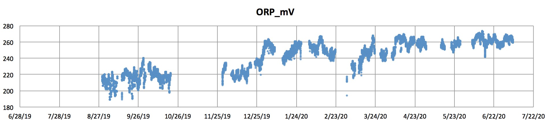
Figure 16 - Temporal evolution of the oxidation-reduction potential. Its average was 242 mV with a low fluctuation range between 189 and 273 mV, with a decrease in March, a plate from April 2020, and little vertical variability (≤ 10 mV).

Figure 17 - Temporal evolution of the dissolved oxygen saturation level. On average, the water column is very well oxygenated (98%), with an amplitude between 67 and 119 %. In general, the vertical variability vertical variability is low (≤ 10%). The minimum value (65%) occurred on January 15 at the bottom.
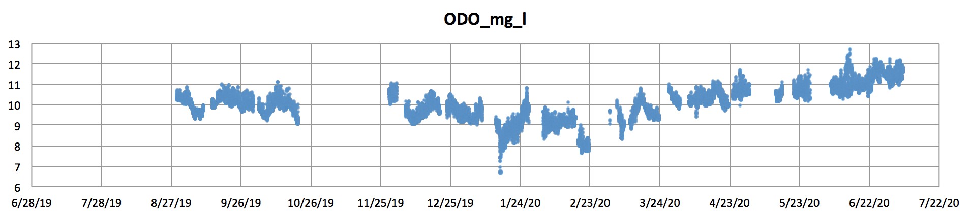
Figure 18 - Temporal evolution of the dissolved oxygen concentration in the water column, identical to OD%. It fluctuated between 6.6 and 12.7 mg/L with an average of 10.0 mg/L, i.e. a very good oxygenation in the whole column, considering the altitude. He lowest values occur in January-February, the rainy season. The vertical variability is ≤ 1 mg/L.
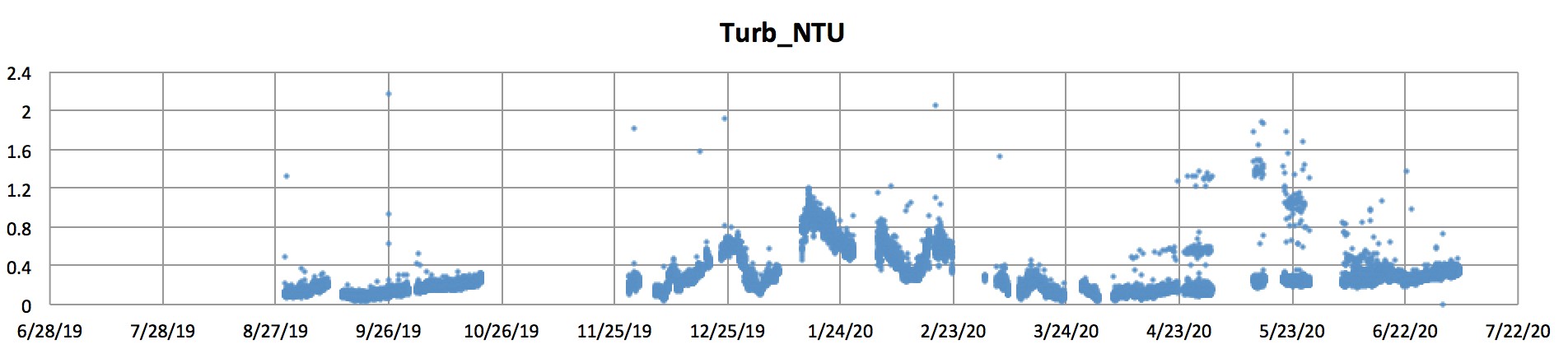
Figure 19 - Temporal evolution of turbidity. It fluctuated between 0.03 and 2.2 NTU. During the dry season turbidity remained ≤ 0.3 NTU. Increased during the rainy season (January-February) up to 1.2 NTU on January 15. In March-April it remained ≤ 0.3 NTU. Then in May there were episodes of high turbidity (1.49 NTU on 5/14, 1.88 NTU on 5/15, and 1.07 NTU on 5/23). On average, vertical variability was low ≤ 0.4 NTU.

Figure 20 - Evolution of phytoplankton chlorophyll-a concentration (RFU = Relative Fluorescence Unit). Chlorophyll-a remained low during the dry season being ≤ 0.7 RFU or ≤ 5.6 µg/L. It increased during the rainy season (January-February) to 2.8 RFU or 22.4 µg/L (corresponding to a mesotrophic state, according to the open trophic classification of the OECD, 1982) on January 15, 2020, then decreased again. Vertical variability was ≤ 0.5 RFU or ≤ 4 µg/L.
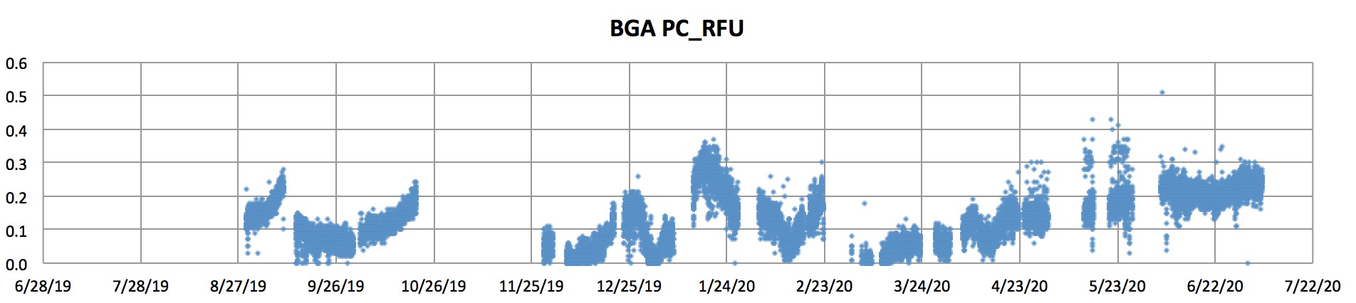
Figure 21 - Evolution of the concentration of phycocyanin, an accessory photosynthetic pigment of cyanobacteria. It varied between 0.01 and 0.51 RFU, being≤ 0.2 RFU in dry season, and up to 0.38 RFU (15/01) in the rainy season (January-February), with a vertical variability ≤ 0.1 RFU.
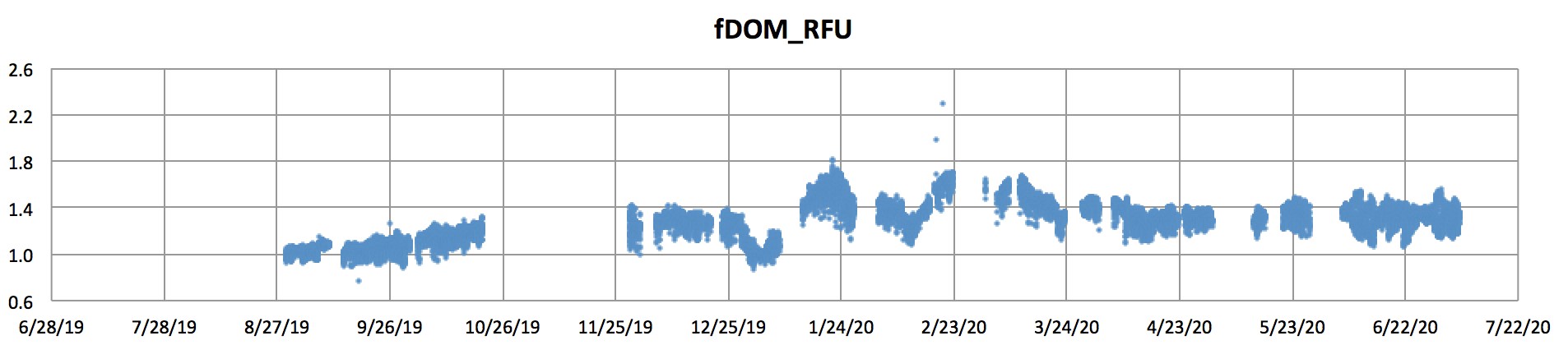
Figure 22 - Evolution of the concentration of fluorescent dissolved organic matter fDOM. It varies between 0.8 and 2.7 RFU (minimum-maximum). It did not exceed 1.3 RFU in the dry season, while it reached 1.8 RFU in the rainy season (January-February). Vertical variability is ≤ 0.2 RFU.
Temporal evolution of water quality at 1 m depth for 2 years
[file = SondeHourly_270619-230721.csv , n = 26,097 observations].
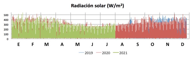
The data presented are raw data, with an acquisition frequency of 30 min. In order to make inter-annual comparisons, we have superimposed the data for the 2nd semester of 2019, the 1st and 2nd semesters of 2020 and the 1st semester of 2021 on a time scale from January (E) to December (D).
Table 1 - Data variability over two years of observation (06/27/2019 to 07/23/2021). Variables: Temp = temperature; Conductivity = conductivity; ORP = oxidation-reduction potential; DO% = % saturation in dissolved oxygen; DO = Dissolved Oxygen; Turbidity = Turbidity; RFU = Relative Fluorescence Unit; Chl-a = Chlorophyll-a, 1 RFU = 8 µg/L; BGA PC = Cyanobacterial Phycocyanin, 1 RFU = 1 µg/L; fDOM = fluorescent dissolved organic matter; Depth = depth of YSI EXO2 probe, Statistics: Mean = Average; Max = Maximum; Min = Minimum; Median = Median; Stdev = Standard deviation; SE = Standard Error (= Stdev/root(number of observations)). *pH sensor decalibrated during 2021. Replaced on 02/12/2019 as of which values are reliable. **ORP outlier. Values Reliable DO values as of October. ***Due to the YSI EXO2 sonde occasionally staying on the bottom (~10 m), the average and median depths are 1.28 m, however close to the programmed 1.0 m.

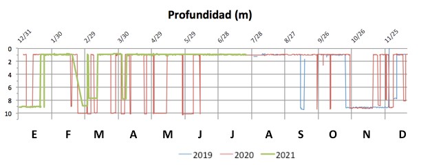
Figure 1 - Temporal evolution of the YSI EXO2 sonde immersion depth (programmed to stay at 1 m depth for measurements every 30 min) during the two years of monitoring. On several occasions the sonde stayed close to the bottom (dammed by drifting fishing nets; by the depth gauge control; or by unknown causes; we fixed the problem in 2021 when it was much less frequent). So, care must be taken to consider these events in interpreting the data.
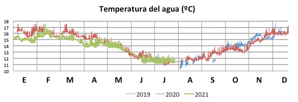
Figure 2 - Temporal evolution of water temperature at 1 m depth (except for some periods during which it was at the bottom; see previous figure). The temperature follows a perfectly parabolic curve parabolic curve, with a maximum of 17.7 ºC from January to March, and a minimum of 10.3 ºC in June-July. The average for the period was 14.2 ºC and the median was 14.4 ºC. During the first half of the year, the temperature was slightly higher (≤ 1 ºC) in 2020 relative to 2021.
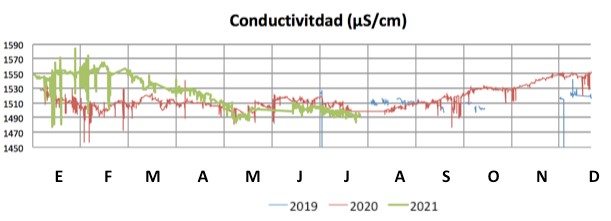
Figure 3 - Temporal evolution of conductivity (in µS/cm) at 1 m depth. On average it has remained at 1,455 µS/cm, except between October and November when the YSI EXO2 sonde was trapped at the bottom, reaching 1,176-1,258 µS/cm (not visible in the graph). This could suggest the presence of fresher water at the bottom. From January to April, the conductivity was higher in 2021 relative to 2020 during the same period. We do not know the cause of this phenomenon: could it be higher evaporation, lower rainfall and/or lower water level in 2021?
.
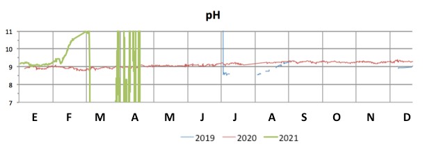
Figure 4 - Temporal evolution of pH at 1 m depth. From June to November 2019, we had a decalibrated sensor (its drift is observed) that was replaced by a new one on 10/12/2019, from when the measurements were reliable. The pH fluctuated between 8.75 and 9.21, with an average of 9.00 during 2020. However, as of February 2021, the sensor was again decalibrated and it was not possible to calibrate it at all. So since February 2021 we have no pH data (nor ORP data for that matter). The sensor was ordered; however, due to the shortage of components during the pandemic, it only arrived on September 28, 2021. It will be installed in October.
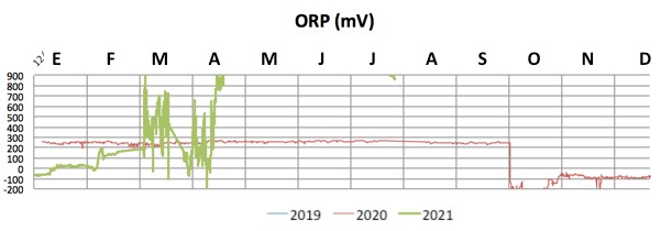
Figure 5 - Time evolution of the oxidation-reduction potential (ORP) in millivolts at 1 m depth. The sensor was recalibrated in October 2019. However, the data were only reliable from January 2021 when they fluctuated between 190 and 270 mV, averaging 241 mV. In 2021, the data has to be discarded. The sensor will be replaced in October 2021.

Figure 6 - Temporal evolution of the percentage saturation of dissolved oxygen at 1 m depth. The sensor was recalibrated in October 2019. As of January 2020, it fluctuated between 67 and 114%, with an average of 98%. This behavior represents a very good level of oxygenation, in equilibrium with the atmosphere. Cycles (oscillations) of 2-4 weeks are observed. A higher oxygenation of up to up to 20% more during 2020 relative to 2021, except from October-December 2020 when oxygenation was lower by up to 20% to 2019 oxygenation. Higher oxygenation may also result from higher micro-algae biomass due to higher photosynthetic intensity.

Figure 7 - Temporal evolution of dissolved oxygen concentration at 1 m depth. Of course, it follows the same pattern as the % saturation in dissolved oxygen (%DO) in Fig. 6. For the same reason, the data are reliable as of October 2019. From October to December 2019 it fluctuated between 8.5 and 11.0 mg/L. From January 2020 it ranged between 7.5 and 11.0 mg/L, with periods of 2-4 weeks. From March 2020, it gradually increased to 12.0 mg/L in June. This corresponds to a good level of oxygenation, given the altitude of the lake. Dissolved oxygen concentration was higher in 2020 by up to 2 mg/L relative to 2021, except from October to December when dissolved oxygen was lower than in 2019. As for %DO it may result from higher biomass/photosynthesis of micro-algae.
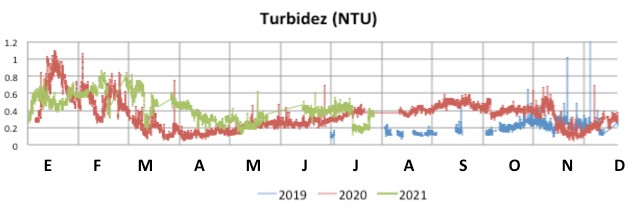
Figure 8 - Temporal evolution of turbidity at 1 m depth. In the dry period (until November) it remained between 0.1-0.6 NTU. It increased in the rainy period (December-February). From January 2020, it reached 1.1 NTU, then gradually decreased with oscillations until reaching 0.2-0.4 NTU at the end of April 2020. From June onwards, it increased slightly. The average is 0.34 NTU and the median is 0.32 NTU, with fluctuations between 0.08 and 4.02 NTU. In other words, the water is very clear. It can be noted that the pattern of turbidity evolution follows the pattern of chlorophyll-a concentration (Fig. 9). In other words, the turbidity mainly reflects the biomass of phytoplankton (not suspended mineral particles).
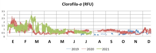
Figure 9 - Temporal evolution of total chlorophyll-a concentration (in RFU) at 1 m depth. During the dry period, it remained between 0.2-1.0 RFU (according to the calibration with the FluoroProbe bbe probe presented in Annex 5 of the 5th Quarterly Report, one has to multiply NTU x 8 to obtain µg/L), i.e. equivalent to 1.6-8.0 µg/L (oligo- to mesotrophic). In the rainy period in January-February (due to nutrient inputs from river runoff, in addition to atmospheric inputs from aerosols) it increased between 0.5-2.8 RFU, i.e. equivalent to 4.0-22.4 µg/L (predominantly mesotrophic-eutrophic). During the annual cycle, chlorophyll-a fluctuated between 0.1-3.0 NTU (i.e. 0.8-24.0 µg/L), averaging 0.34 RFU (i.e. 2.72 µg/L). In comparison, during 1979-1980, for all of Minor Lake, chlorophyll-a concentrations did not exceed 0.34 RFU (i.e., 2.72 µg/L). in chlorophyll-a did not exceed 0.5 µg/L in the dry period and 2.0 µg/L in the rainy period, with a maximum of 5.0 µg/L (Lazzaro, 1981). This means that, compared to 1979-1980, the current Chl-a concentration is up to x 16 higher during the dry period, and up to x 11 higher during the rainy period, ... compared to 40 years ago. This demonstrates the significant increase in the biomass of microalgae in response to the combination of the effects of climate change with several decades of massive nutrient inputs from pollution from the urban area of El Alto via the Katari watershed.

Figure 10 - Temporal evolution of the concentration of phycocyanin (photosynthetic pigment of cyanobacteria) at 1 m depth. During this 2-year period, the phycocyanin remained below 0.4 RFU, with a maximum of 2.9 RFU. According to the manufacturer's YSI calibration, 1 RFU = 1 µg/L phycocyanin. The average was 0.78 RFU (=0.78 µg/L) that is a relatively low concentration. The concentration was slightly higher during the 2nd half of 2020 relative to 2019. It was slightly higher during the 1st half of 2021 relative to 2020, with a delayed peak at the beginning of March 2021 (0.4 RFU) extended until the beginning of April 2021, relative to the peak of 0.32 RFU only during January 2020. This suggests poorer quality waters during the 2021 rainy period, as well as a gradual increase in the contribution (~doubling) of cyanobacterial biomass from 2019 (≤ 0.2 RFU) to 2021 (≤ 0.4 RFU). Meanwhile, the ratio of cyanobacterial biomass to total phytoplankton biomass decreased slightly from 0.15/0.5 = 30% in 2019 to 0.2/1.0 = 20% in 2021. However, we need the data for 3 full years to confirm this calculation. A ratio of 20-30% is quite high. It suggests keeping a high and permanent vigilance, because if conditions become favorable, cyanobacteria can quickly proliferate and generate blooms (= Blooms) that can become recurrent every year. The damage (mortality of fish, frogs and waterfowl) would be irreparable and repeated in the long term, since cyanobacterial blooms would be impossible to control in Lake Titicaca. In fact, the Titicaca has no herbivorous organisms (neither fish nor zooplankton) capable of grazing them effectively, nor wastewater treatment plants (WWTPs) capable of retaining the nutrients used by the algae for their growth. Nutrients used by the algae for their growth. Even if cattails are natural biological filters of nutrients and pollutants, alone, in the absence of WWTPs, they are not capable of controlling the biological discharges of a population of 1.2 M inhabitants of the urban area of El Alto. In order to have beneficial effects, cattails (and wetlands in general) have to be associated as a complementary treatment to WWTPs, as shown in the following table by WWTPs, as is universally practiced throughout the world.

Figure 11 - Temporal evolution of fluorescent dissolved organic matter (fDOM) concentration at 1 m depth. During the dry period it varied between 0.9-1.5 RFU. It increased slightly during the rainy period from 1.7 RFU in February 2020 to 2.1 RFU in November 2020. This increase in February and November resulted from organic matter inputs from the rivers, particularly from the Katari basin. from the Katari watershed, via the Cohana and Sehuenca rivers joining in the Cumana Lagoon, which flows into Cumana Bay. Counter-intuitively to what was thought about the pandemic and quarantine period in 2020, the concentration of organic matter (fDOM) was much higher in 2020 than in the second half of 2019 and the first half of 2021. In fact, the population did not stop contributing to the organic pollution of rivers and lakes. Contrary to what the press wanted to convince us, no significant improvement in the water quality of the Lesser Lake was observed in 2020. Even if discharges of organic matter organic matter would have stopped completely in 2020 (impossible situation), the organic matter already deposited for decades with the polluted sediments would not have disappeared in one year with the action (= mineralization) of the microbial loop. In conclusion, it is imperative to maintain permanent long-term monitoring, since without the implementation of new WWTPs, there are no mechanisms to eliminate such massive nutrient discharges of nutrients and organic matter that benefit micro-algal blooms.
Temporal evolution of water quality along vertical profiles between 1 and 10 m depth every 2 hours.
[file = PFL_Step_270619-280721.csv, n = 55,350 observations].
The time scale (horizontal axis) of the graphs is indicated with monthly divisions.
Table 2 - Variability of the data over the two years of observation (06/27/2019 to 07/28/2021). For variable abbreviations and statistics see Table 1. The pH data are not are indicated here because the removable sensors have reached the end of their useful life (they have to be replaced after 6-12 months), so we have not been able to recalibrate them and the 2021 data are not usable. The same is true for the ORP data. The replacement sensors took several months to arrive. Replacement will take place in October or November 2021.
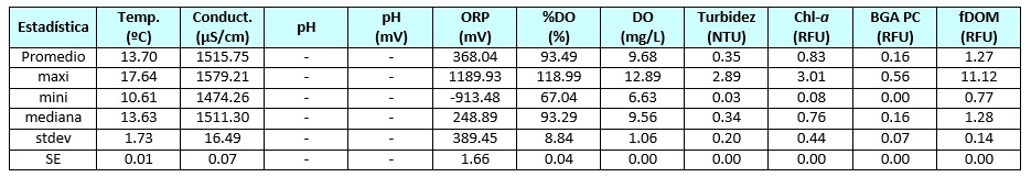
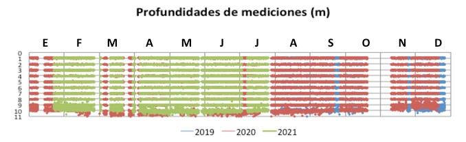
Figure 12 - Vertical profiles at every meter between 1 and 10 m depth performed daily at every two hours (2:00, 4:00, 6:00,..., 22:00, 24:00; i.e. 12 daily profiles). In 2019 and 2020, on several several occasions the sonde was stranded near or on the bottom dragged by drifting fishing nets, or for unknown causes. From 2021 onwards this occurred sparingly.
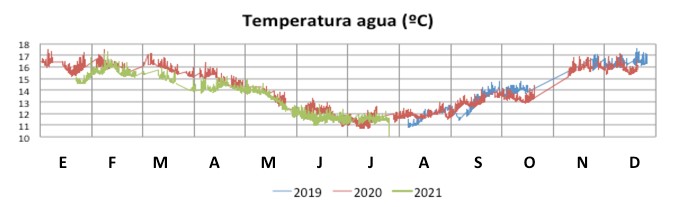
Figure 13 - Time evolution of vertical temperature profiles between 0 and 10 m depth. The vertical amplitude of each measurement (≤ 1 ºC) indicates the difference in temperature between the surface and the bottom. The data follow a parabola curve (in relation to the seasonal variation of the sun's height above the horizon). During the 1st half of the year, the 2020 temperature was slightly higher (≤ 1ºC) at the higher (≤ 1°C) relative to 2021. During the 2nd half of the year, 2019 and 2020 temperatures were quite similar. In the rainy seasons (December to March) temperatures reached 16-17 ºC, while in the dry seasons (June to August) they dropped to 12-11 ºC.

Figure 14 - Conductivity evolution. In the 2-year period, the average was 1,515 and the median 1,511 µS/cm. During the rainy season the conductivity was surprisingly slightly higher (up to 1,560 µS/cm).; the opposite would be expected because of the concentration of salts when the water level drops (~1.0-1.5 m) with drought. In 2020, the conductivity remained fairly constant throughout the year except for the year except from October to December when it increased to 1,550 µS/cm. During the 1st half of the year, 2021 conductivity was slightly higher (~1,550-1,560 µS/cm) than in 2020. During the 2nd half of the year, conductivity was slightly higher in 2020 (~1,550 µS/cm) than in 2019 (~1,520 µS/cm).
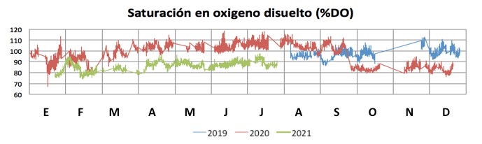
Figure 15 - Temporal evolution of the dissolved oxygen saturation level (%DO). On average, the water column is very well oxygenated (> 93%), with an amplitude between 67 and 119 %. In general, the vertical variability is low (≤ 10%). Oxygenation during 2020 was higher than 2021, except from October to December when it was lower than 2019, around 15%.

Figure 16 - Time evolution of dissolved oxygen concentration (DO, mg/L) in the water column. The pattern is identical to that of the DO%. During the two years, it fluctuated between 6.6 and 12.9 mg/L with an average of 9.7 mg/L. an average of 9.7 mg/L, i.e. very good oxygenation throughout the column, taking into account the altitude. The lowest values arose in January-February (~8-9 mg/L), in rainy seasons, with maxima in dry seasons (June-February), dry seasons (June-August, ~10.0-12.9 mg/L). Vertical variability was low ≤ 1 mg/L. The concentration was higher in 2020 (~1.5 mg/L) compared to 2021. Except in October-December, when it was higher in 2019 relative to 2020.
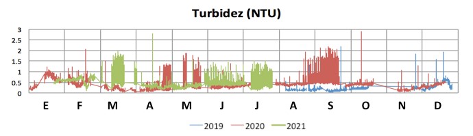
Figure 17 - Temporal evolution of turbidity. It fluctuated between 0.03 and 2.9 NTU. During the dry season, turbidity remained ≤ 0.3 NTU. Increased during the rainy season (January-February) up to ~1.5-2.0 NTU. From March to September, there were episodes (for 1-3 weeks) of higher turbidity (~1.5-2.0 NTU). On average, vertical variability was low ≤ 0.4 NTU. Turbidity in 2020 was higher than that of 2019 during the 2nd half of the year, and that of 2021 during the 1st half of the year.
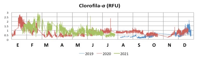
Figure 18 - Evolution of phytoplankton chlorophyll-a concentration (in RFU = Relative Fluorescence Unit; 1 RFU = 8 µg/L). Chlorophyll-a remained low during the dry season (April-November) being. ≤ 0.7 RFU or ≤ 5.6 µg/L. It increased during the rainy season (January-February) to 2.8 RFU or 22.4 µg/L (corresponding to a mesotrophic state, according to the open trophic classification of the OECD, 1982). The vertical variability was ≤ 0.5-1.0 RFU or ≤ 4-8 µg/L, being higher near the bottom, with a surface inhibition in the first meter where solar radiation, especially ultraviolet radiation is too intense and harmful to microalgae. During the 1st half of the year, chlorophyll-a was higher in 2021 (~+1µg/L) relative to 2020. The peak occurred in mid-January 2020 (2.7 RFU = 21.6 µg/L) and later at the end of February 2021 (3.0 RFU = 24.0 µg/L). It should be noted that in this northeastern region of Lake Minor in 1979-1980, the chlorophyll-a did not exceed 3.0 µg/L, i.e. characteristic of an oligotrophic state (Lazzaro, 1981). Thus, although it is not noticeable at first sight (without the use of a probe), the phytoplankton biomass has increased up to 8 times in the last 40 years, as a consequence of the greater availability of nutrients from nutrient inputs from the sea. Nutrient availability from anthropogenic inputs (mostly from the urban region of El Alto via the Katari basin) combined with the effects of global warming, which magnify eutrophication.
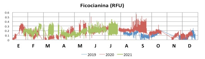
Figure 19 - Evolution of the concentration of phycocyanin, an accessory photosynthetic pigment characteristic of cyanobacteria. It varied between 0.01 and 0.56 RFU (1 RFU = 1 µg/L), with an average and median of 0.16 RFU (1 RFU = 1 µg/L). I tended to have higher concentrations during the dry season, particularly in June-July and September, with periods of 2-3 weeks with sustained higher values up to 0.45-0.55 RFU and variability of up to 0.3 RFU between surface and background. During 2020, the concentration was generally higher (~+0.1 RFU) during the 1st half of 2021 relative, and during the 2nd half of 2021 relative a 2019. Two peak periods are noted, one in January-February 2020-2021 (peak rainfall) and the other in July (peak of the dry season) and end of August-September (time of peak winds). This suggests that massive inputs of nutrients and their vertical mixing by winds, respectively, stimulate the increase of cyanobacteria. When comparing the phycocyanin graph with the chlorophyll-a graph, it is noted that in general the phycocyanin concentration represents 10% to 20% of the chlorophyll-a concentration. This encourages us to keep an eye on the dynamics of the cyanobacteria (phycocyanin) which have the capacity to rapidly generate blooms (= proliferations or blooms) when conditions are favorable, which can be extremely harmful and could then occur on a recurring basis every year.
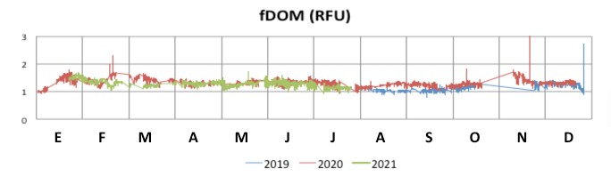
Figure 20 - Evolution of the concentration in fluorescent dissolved organic matter fDOM. It varied between a minimum of 0.8 RFU and an exceptional maximum of 11.1 RFU, with mean and median of 1.3 RFU. Generally, it remained low between 1-2 RFU, stably throughout the year. Its vertical variability was ≤ 0.2 RFU. We can conclude that in this relatively deep zone (11 m) for the Bolivian sector of the Minor Lake ( < 5 m), the concentration in dissolved organic matter is low.